2:Loss Measuring Concepts
Optical Loss Measuring Concepts
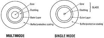
Fig 2.1: Cross-section of typical single mode and multimode fibers.
In both case, the glass diameter is 125u, and the diameter
including a protective acrylate plastic coating is 250u.
Glass fiber used for data communications comes in 2 general types:
- Single mode fiber is used to transmit 1270 – 1650 nm light over long distances and high data rates, most commonly at 1310 and 1550 nm. DWDM (Dense Wavelength Division Multiplexing) systems operate in the C, S and L bands in the region of 1450 – 1650 nm, and CWDM (Corse Wavelength Division Multiplexing) systems operate over 1270 – 1610 nm. A single ray of light travels down the fiber core, with a mode field diameter of about 9.5 um. Single mode fiber comes in varying grades typically designed to optimise loss, chromatic dispersion and polarisation mode dispersion, and with varying levels of water peak performance at 1383 nm. Current developments are aimed at improved bend tolerance for FTTX applications. Wavelengths below 1270 nm are transmitted as multimode light by standard 9.5 um core fiber, and specialist small-core fiber is required to achieve single mode operation below 1270 nm. Wavelengths above 1625 nm are more heavily attenuated.
Typical singlemode loss is 0.35 dB / Km at 1310 nm, which with a typical link loss of 20 dB, gives a maximum link length of 57 Km. The ability to achieve such long transmission distances between repeaters or amplifiers is a major factor in it’s success.
- Multimode fiber is commonly used to transmit light at 850 and 1300 nm for shorter distances and moderate data rates. Multiple rays of light travel down the core, which has a diameter of 62.5 um or 50 um. Modern 50u core types have higher bandwidth and couple well with VCSEL lasers. Older 62.5u core types give better coupled power from an LED, but lower bandwidth. Multimode fiber comes in varying grades typically designed to optimise bandwidth or pulse dispersion. The core has a graded refractive index structure, to reduce pulse dispersion of the various light rays. It is therefore more complicated to manufacture than single mode fiber.
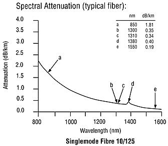
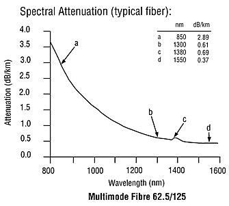
Fig 2.2: Typical attenuation graphs for multimode and single mode loss. Note that the loss is sensitive to wavelengths
 Fig 2.3: Fibre Optic Transmission Windows
Loss
The above graphs show typical loss when the glass is mechanically unstressed. Additional loss will be created under stress, and this is termed “microbend loss”. Microbend loss is typically caused by: kinking, tension, heat or cold, crushing, winding onto a drum, excessively sharp bending, defective manufacture, or poor cable design. The above graph also fails to show rapidly increasing attenuation above about 1625 nm.
Multimode loss measuring is inherently more uncertain than singlemode measuring, since there are additional variables as follows:
- Attenuation varies depending on the power distribution across the fiber core. So loss measuring should be performed with a defined modal distribution to ensure that results are repeatable with different meters.
- The LED sources typically used have uncertain characteristics. The center wavelength, spectral width and modal power distribution in the coupled fiber can vary significantly, resulting in varying loss measurements. So the characteristics of sources should comply with various standards.
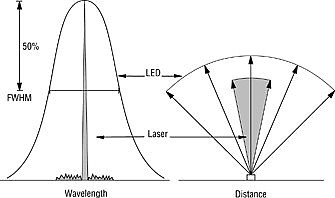
Fig 2.3: A comparison of the spectral and spatial distribution of Lasers and LEDs.
Single mode loss tends to be more stable than multimode, since multi-mode transmission characteristics create instantaneously changing loss characteristics. This is readily observed during practical measurement, where moving multimode patch leads around creates obvious measurement variations.
The loss budget refers to the calculated allowable loss before a link stops working. This is usually determined as a function of transmitter power, receiver sensitivity, and a required reserve margin. The expected losses of individual segments of the link are then estimated, along with a nominal margin to allow for degradation and maintenance. On long or high speed links, estimating these effects for optimum overall lifetime performance, requires considerable skill and experience. On short or low speed links, the link loss is usually much less critical , so this is much easier, or it may be defined in appropriate standards.
Unlike the loss budget, the optical margin refers to the change in actual loss that an operating link can suffer before it stops working. Note this could be either an increase or decrease in loss.
Single mode loss is more sensitive to fiber bending or mechanical stress at wavelengths above 1480 nm. It is therefore common to perform additional measurements on single mode at 1550 nm, as a means of verifying the installed performance, even if the operational system is to be used at 1310 nm.
High bit rate systems may have a quite small working tolerance for the receiver power level. This results in a requirement of tighter absolute power measurement accuracy. For example, low bit rate systems may have a loss budget of 0 – 25 dB, whereas high speed LAN systems may have a loss budget of only 0 – 2.5 dB.
Other components in the transmission path will introduce more loss, for example:
| Component | Loss | |
| Single mode | 1310 nm | 0.33 – 0.35 dB/km |
| 1550 nm | 0.17 -0.22 dB/km | |
| Multimode | 850 nm | 2.5 – 3.0 dB/km |
| 1310 nm | 0.7 – 0.8 dB/km | |
| Connectors | 0.1 – 0.75 dB | |
| Fusion splices | 0.1 – 0.15 dB | |
| Mechanical splices | 0.1 – 1 dB | |
| Switches | 0.1 – 1.5 dB | |
| Couplers | 1 – 21 dB (power splitter) | |
| Isolators | 0.5 – 5 dB | |
These figures are very approximate: the exact value will depend on the equipment selected in your application. Note in particular that connector losses are quite uncertain: the same pair of connectors will show a randomly varying loss when mated on different occasions. The connector specification will show the average value, which by definition will often not be achieved. Connector loss is better understood by using a statistical mean and standard deviation approach.
Loss Measurement Techniques
To accurately measure the end to end loss of a system, it is usual to test at the target wavelength using an LTS, or source and meter.
End to end loss cannot be reliably measured with optical time domain reflectometry, since an OTDR works by mathematical deduction based on a number of assumptions. To accurately measure a splice or connector point loss with an OTDR, a measurement must be made from each end direction, and then averaged. This is not always simple to do. An OTDR excels at identifying the location of an event, and measuring length.
The accuracy of typical loss measurement methods with a source and meter are usually dominated by these factors:
- Source power levels drift over time, so a short measurement time is preferable.
- Source wavelength tolerance may be an accuracy limiting factor over long distances.
- Optical power meter absolute accuracy is not as good as that for other measurement metrologies such as mass, length or electrical.
- Somehow a source reference measurement must be known or obtainable, often while being with the power meter, many Km from the source, at the other end of the link.
- Loss in the same link may be different if measured in different directions. This may be the result of mis-matching or incorrect optical or core diameter characteristics. In practice, mismatched fibre cores can be picked up if two correctly selected test cords are used during measurement.
- Bi-directional loss method is the practical solution for all of the above issues.
- Because of wavelength sensitivity, measurement should be performed at the same wavelength as the operational system. Other wavelengths may be tested as well.
The requirement of better accuracy has made the bi-directional two-wavelength method the preferred and practical solution. With a pair of modern two-way LTS, the complete analysis can be completed in a few seconds. This measurement method requires either two LTS, or two sources and two meters.
To summarize, measurements using two-way averaging have the following benefits:
- The elapsed time between taking a reference and second measurements may be very short, so only the short term source stability matters.
- Meter absolute accuracy is irrelevant.
- Core diameter or other optical mismatches will always be found.
- The highest possible accuracy is always achieved.
- If a sub-standard test cord is used, errors are halved
- A low level of operator skill is required.
Effect of Testing Wavelength Uncertainty on loss measurements
Most test sources have a significant practical wavelength tolerance. For example many “1310 nm laser sources” may have a wavelength tolerance of ± 30 nm. Add ± 5 nm for temperature variations, resulting in an actual wavelength of 1310 ± 35 nm. If an LED is used, the FWHM spectral width is probably ± 50 nm, resulting in the possibility of light being transmitted anywhere in the band of 1300 ± 85 nm, eg from 1215 – 1385 nm. Fiber loss characteristics may vary quite significantly over these extremes.
As a result of source wavelength uncertainty, there may be some variation between the conditions under which a system is tested, and actual in-service conditions. To put this into perspective, @ 1310 nm on a link of say 50 Km, the link attenuation uncertainty caused by a tolerance of ± 30 nm would be about ± 0.95 dB.
In some older systems, or in a research environment, possible effects due to cladding mode transmission may need to be assessed, however with modern cladding mode stripping fiber, these effects can usually be ignored.
Summary
- Loss should always be measured at the same wavelength band as the operational system.
- Loss is ideally measured from both directions.
- Loss should be measured with a source and meter, or LTS.
- Multimode loss measurements are intrinsically inaccurate compared to those on single mode systems. Adherence to relevant standards may be advisable, to ensure repeatability.
- Cladding modes can occasionally cause measurement errors in unusual circumstances.
- The effects of wavelength variations within a wavelength window should be evaluated, both on measurement accuracy, and also on the installed system.
- An allowance for future degradation should be made, to ensure reliable performance. This is called the optical margin.